Overview of Data Types in R
R Data Types: The Foundation of Data Analysis
In R, everything is an object, and each object has a specific data type. Understanding these data types is crucial for effective data manipulation and analysis in business contexts.
Basic Data Types in R
| Data Type | Description | Example | Business Use Case |
|---|---|---|---|
| Numeric | Decimal numbers (real numbers) | 12.5, 3, -4.7 | Financial figures, sales data, percentages |
| Integer | Whole numbers without decimals | 5L, -3L, 100L | Count data, inventory levels, customer counts |
| Character | Text or string values | “Hello”, “Product A”, “New York” | Product names, customer segments, locations |
| Logical | Boolean values (TRUE/FALSE) | TRUE, FALSE | Binary classifications, condition checks |
| Complex | Complex numbers with real and imaginary parts | 3+2i | Advanced mathematical modeling |
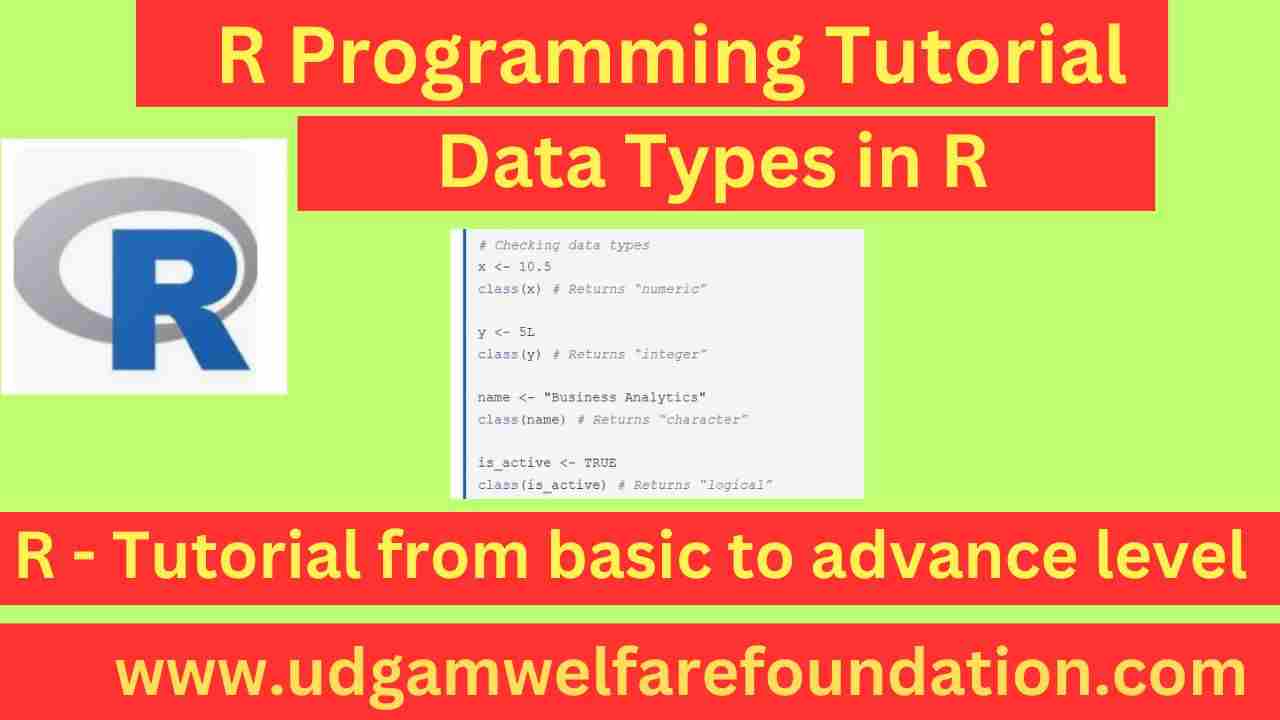
Checking Data Types
You can check the data type of any object in R using the class() or typeof() functions:
x <- 10.5
class(x) # Returns “numeric”
y <- 5L
class(y) # Returns “integer”
name <- "Business Analytics"
class(name) # Returns “character”
is_active <- TRUE
class(is_active) # Returns “logical”
Data Structures in R
While data types define the kind of data, data structures define how data is organized. The main data structures in R are:
- Vectors – One-dimensional arrays that can hold elements of the same data type
- Matrices – Two-dimensional arrays with rows and columns
- Data Frames – Tabular data structures with rows and columns (similar to Excel spreadsheets)
- Lists – Collections of objects that can be of different data types
- Factors – Special vectors used to represent categorical data
Vectors in R
Vectors are the most basic data structure in R. All elements in a vector must be of the same type.
# Numeric vector
sales <- c(12500, 13800, 14200, 11900, 15600)
# Character vector
products <- c(“Laptop”, “Tablet”, “Smartphone”, “Monitor”)
# Logical vector
in_stock <- c(TRUE, FALSE, TRUE, TRUE)
# Accessing vector elements
sales[1] # First element: 12500
products[2:4] # Elements 2 to 4: “Tablet”, “Smartphone”, “Monitor”
Data Frames for Business Analysis
Data frames are the most commonly used data structure in R for business analysis. They resemble Excel spreadsheets or database tables.
sales_data <- data.frame(
Product = c(“Laptop”, “Tablet”, “Smartphone”, “Monitor”),
Q1_Sales = c(12500, 9800, 15600, 4200),
Q2_Sales = c(13800, 10200, 16800, 4800),
Growth = c(TRUE, TRUE, TRUE, TRUE)
)
# View the data frame
print(sales_data)
# Accessing data frame elements
sales_data$Product # Access the Product column
sales_data[1, ] # First row
sales_data[, 2] # Second column
sales_data[2, 3] # Element at row 2, column 3
Factors for Categorical Data
Factors are used to represent categorical variables in R. They are especially useful in statistical modeling and data analysis. A factor stores categorical data as integer codes associated with a set of levels (unique category labels).
customer_segment <- factor(c(“Premium”, “Standard”, “Basic”, “Premium”, “Basic”))
# View the factor
print(customer_segment)
# Check levels
levels(customer_segment)
# Changing factor levels
levels(customer_segment) <- c(“Basic”, “Standard”, “Premium”)
[1] Premium Standard Basic Premium Basic
Levels: Basic Standard Premium
Example: Factor vs Character Vector
The following example compares a simple character vector with a factor created from it. You’ll see that R internally stores factors as integer codes associated with level labels.
fruits_vec <- c(“Apple”, “Banana”, “Apple”, “Cherry”)
# Factor
fruits_fac <- factor(fruits_vec)
# Compare
fruits_vec
fruits_fac
str(fruits_fac)
[1] “Apple” “Banana” “Apple” “Cherry”
[1] Apple Banana Apple Cherry
Levels: Apple Banana Cherry
Factor w/ 3 levels “Apple”,”Banana”,”Cherry”: 1 2 1 3
Practical Examples for Business Analysis
Example 1: Sales Data Analysis
Let’s create a simple sales analysis using different data types and structures:
# ‘regions’ is a character vector that stores the names of the sales regions.
regions <- c(“North”, “South”, “East”, “West”)
# ‘q1_sales’ stores the sales values for each region during Quarter 1.
q1_sales <- c(45000, 52000, 38000, 61000)
# ‘q2_sales’ stores the sales values for each region during Quarter 2.
q2_sales <- c(48000, 54000, 41000, 65000)
# ——————————————————-
# Calculate growth and growth rate
# ——————————————————-
# ‘growth’ calculates the difference between Q2 and Q1 sales for each region.
growth <- q2_sales - q1_sales
# ‘growth_rate’ calculates the percentage growth for each region.
growth_rate <- (growth / q1_sales) * 100
# ——————————————————-
# Create a data frame to summarize the information
# ——————————————————-
sales_summary <- data.frame(
Region = regions,
Q1_Sales = q1_sales,
Q2_Sales = q2_sales,
Growth = growth,
Growth_Rate = growth_rate
)
# ——————————————————-
# View the summary
# ——————————————————-
print(sales_summary)
# ——————————————————-
# Find the region with the highest growth
# ——————————————————-
max_growth_idx <- which.max(sales_summary\$Growth)
top_region <- sales_summary\$Region[max_growth_idx]
cat(“Region with highest growth:”, top_region)
Example 2: Customer Segmentation
Using factors and data frames for customer segmentation analysis:
customer_id <- 1:10
segment <- factor(c(“Premium”, “Standard”, “Basic”, “Premium”, “Standard”,
“Basic”, “Premium”, “Basic”, “Standard”, “Premium”))
purchase_amount <- c(250, 120, 80, 300, 150, 70, 280, 90, 130, 320)
# Create customer data frame
customers <- data.frame(
ID = customer_id,
Segment = segment,
Purchase = purchase_amount
)
# Calculate average purchase by segment
avg_purchase <- tapply(customers\$Purchase, customers\$Segment, mean)
print(avg_purchase)
# Count customers by segment
segment_counts <- table(customers\$Segment)
print(segment_counts)
Key Takeaways
- R has five basic data types: numeric, integer, character, logical, and complex
- Vectors are the fundamental data structure in R and must contain elements of the same type
- Data frames are the most important structure for business analysis, resembling spreadsheet data
- Factors are used to represent categorical variables, essential for statistical modeling
- Understanding data types is crucial for proper data manipulation and analysis in business contexts
In the next session, we will explore data import/export techniques and basic data manipulation in R.