Writing Beautiful Mathematical Equations in LaTeX
Introduction
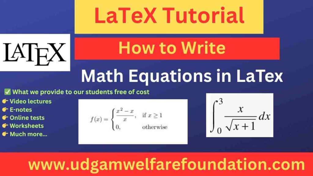
LaTeX is the gold standard for typesetting mathematical equations and scientific documents. Its powerful syntax allows you to create beautiful, precise, and complex mathematical expressions with ease. This guide will teach you how to write stunning mathematical equations in LaTeX, from basic formulas to advanced expressions.
Why Use LaTeX for Equations?
- Precision: LaTeX ensures that your equations are rendered with perfect alignment and clarity.
- Flexibility: Supports everything from simple fractions to complex matrices and integrals.
- Professional Quality: Produces publication-ready equations for research papers, theses, and books.
- Widely Used: The standard tool for mathematicians, physicists, and engineers.
Useful LaTeX Packages for Math Equations in TeXstudio
TeXstudio supports a variety of LaTeX packages that enhance your ability to write mathematical equations. Below are some of the most useful packages for math typesetting:
1. amsmath
The \texttt{amsmath} package is one of the most widely used extensions in \LaTeX{} for typesetting mathematical content. It provides advanced tools that go far beyond the basic math mode. With this package, you can create multi-line equations, align equations properly, insert matrices, and display complex mathematical structures with clarity. It also introduces environments such as \texttt{align}, \texttt{gather}, and \texttt{multline}, which are extremely useful when dealing with step-by-step derivations or long mathematical proofs. In professional and academic writing, \texttt{amsmath} is considered a standard for formatting high-quality mathematical expressions.
\usepackage{amsmath}
Example: Aligned equations
\begin{align*}
    f(x) &= (x+1)^2 \\
         &= x^2 + 2x + 1
\end{align*}
Output:
\[ \begin{align*} f(x) &= (x+1)^2 \\ &= x^2 + 2x + 1 \end{align*} \]
2. amssymb
The \texttt{amssymb} package complements \texttt{amsmath} by providing a wide variety of additional mathematical symbols. It is especially helpful for students, researchers, and teachers who need to use special operators, advanced relation symbols, Greek letters in bold, or set notations such as $\mathbb{R}$ for real numbers. Without \texttt{amssymb}, these symbols would either be missing or difficult to create. It is commonly used in fields like pure mathematics, statistics, and engineering where symbolic representation plays a crucial role. The package is simple to load but adds a great deal of flexibility to any mathematical document.
\usepackage{amssymb}
Example: Special symbols
The set of real numbers is denoted by $\mathbb{R}$.
Output: \(\mathbb{R}\)
3. physics
The \texttt{physics} package is designed to simplify the writing of common physics and calculus notations. It provides shortcuts for derivatives, integrals, vectors, bras and kets, and even norms and commutators. Instead of manually writing lengthy commands, the package allows you to use compact, readable syntax such as \verb|\dv{f}{x}| for derivatives or \verb|\vb{v}| for vectors. This not only saves time but also makes your code more intuitive and easier to revise. Physics students and researchers benefit greatly from this package, as it standardizes notation in scientific documents while keeping the code concise and clear.
\usepackage{physics}
Example: Derivatives
The derivative of \(f(x)\) is \(\dv{f(x)}{x}\).
Output: \(\dv{f(x)}{x}\)
4. bm
The \texttt{bm} package is specifically designed to make mathematical symbols bold, something not easily done in regular \LaTeX{}. While text can be boldfaced with \verb|\textbf{}|, mathematical expressions like vectors, Greek letters, or operators require special handling. The \texttt{bm} package provides the command \verb|\bm{}|, which can be applied to almost any mathematical symbol to highlight it in bold. This feature is especially useful in linear algebra, vector calculus, and physics, where bold symbols typically denote vectors or matrices. It gives authors better control over notation and helps distinguish between scalar and vector quantities in equations.
\usepackage{bm}
Example: Bold vectors
The vector \(\bm{v}\) is defined as \(\bm{v} = \begin{pmatrix} v_1 \\ v_2 \end{pmatrix}\).
Output: \(\bm{v} = \begin{pmatrix} v_1 \\ v_2 \end{pmatrix}\)
5. mathtools
The mathtools package extends amsmath with additional tools for fine-tuning mathematical layouts.
\usepackage{mathtools}
Example: Multi-line equations with improved spacing
\begin{multline*}
    f(x) = a_0 + a_1x + a_2x^2 + \cdots \\
    + a_nx^n
\end{multline*}
Output:
\[ \begin{multline*} f(x) = a_0 + a_1x + a_2x^2 + \cdots \\ + a_nx^n \end{multline*} \]
Basic Equations
LaTeX uses math mode to typeset equations.
Inline equations are enclosed in $...$, while displayed equations use \[...\] or \begin{equation}...\end{equation}.
Inline Equations
Inline equations are used within a line of text. For example, the equation \(E = mc^2\) is written as:
Einstein's famous equation is $E = mc^2$.
Output: Einstein’s famous equation is \(E = mc^2\).
Displayed Equations
Displayed equations are centered and set apart from the text. For example, the quadratic formula:
The quadratic formula is given by:
\[ x = \frac{-b \pm \sqrt{b^2 - 4ac}}{2a} \]
Output:
\( x = \frac{-b \pm \sqrt{b^2 – 4ac}}{2a} \)
Fractions and Roots
Fractions
Fractions are created using the \frac{numerator}{denominator} command.
The fraction \(\frac{3}{4}\) is written as:
$\frac{3}{4}$
Output: \(\frac{3}{4}\)
Roots
Square roots are created using the \sqrt{expression} command.
For nth roots, use \sqrt[n]{expression}.
The square root of 2 is \(\sqrt{2}\).
The cube root of 8 is \(\sqrt[3]{8}\).
Output: \(\sqrt{2}\), \(\sqrt[3]{8}\)
Exponents and Indices
Exponents
Exponents are written using the ^ symbol.
The expression \(x^2\) is written as:
$x^2$
Output: \(x^2\)
Indices
Indices are written using the _ symbol.
The expression \(a_1\) is written as:
$a_1$
Output: \(a_1\)
Sums and Integrals
Sums
Sums are created using the \sum command.
Use _{lower}^{upper} to specify the limits.
The sum \(\sum_{i=1}^{n} i^2\) is written as:
$\sum_{i=1}^{n} i^2$
Output: \(\sum_{i=1}^{n} i^2\)
Integrals
Integrals are created using the \int command.
Use _{lower}^{upper} to specify the limits.
The integral \(\int_{a}^{b} x^2 \, dx\) is written as:
$\int_{a}^{b} x^2 \, dx$
Output: \(\int_{a}^{b} x^2 \, dx\)
Matrices
Matrices are created using the \begin{matrix}...\end{matrix} environment.
For matrices with parentheses, use pmatrix; for brackets, use bmatrix.
The matrix
\[
\begin{pmatrix}
1 & 2 \\
3 & 4
\end{pmatrix}
\]
is written as:
\[
\begin{pmatrix}
1 & 2 \\
3 & 4
\end{pmatrix}
\]
Output:
\[ \begin{pmatrix} 1 & 2 \\ 3 & 4 \end{pmatrix} \]
Greek Letters
Greek letters are commonly used in mathematical equations.
Use the letter’s name prefixed with a backslash (e.g., \alpha, \beta).
The Greek letter \(\alpha\) is written as:
$\alpha$
Output: \(\alpha\)
Advanced Equations
LaTeX can handle complex equations with multiple levels, alignments, and annotations.
The wave equation is:
\[
\frac{\partial^2 u}{\partial t^2} = c^2 \nabla^2 u
\]
Output:
\[ \frac{\partial^2 u}{\partial t^2} = c^2 \nabla^2 u \]
Practical Exercise
Try writing the following equations in LaTeX:
- The Pythagorean theorem: \(a^2 + b^2 = c^2\).
- A definite integral: \(\int_{0}^{\pi} \sin(x) \, dx\).
- A matrix: \[ \begin{bmatrix} 1 & 0 \\ 0 & 1 \end{bmatrix} \]
- The binomial coefficient: \(\binom{n}{k} = \frac{n!}{k!(n-k)!}\).
Solutions:
1. The Pythagorean theorem: $a^2 + b^2 = c^2$

2. A definite integral: $\int_{0}^{\pi} \sin(x) \, dx$

3. A matrix:
\[
\begin{bmatrix}
1 & 0 \\
0 & 1
\end{bmatrix}
\]

4. The binomial coefficient: $\binom{n}{k} = \frac{n!}{k!(n-k)!}$
Tips for Writing Beautiful Equations
- Use Display Mode: For complex equations, use
\[...\]to center and highlight them. - Align Equations: Use the
alignenvironment for multi-line equations. - Add Spacing: Use
\quador\;to add space between elements. - Learn Common Commands: Familiarize yourself with commands for symbols, operators, and structures.
- Practice: The more you write, the more comfortable you’ll become with LaTeX syntax.